Home Science Page Data Stream Momentum Directionals Root Beings The Experiment
Now that we have discovered the Slope of our Line, let us generate the Equation for the Line itself. But first let us look at a computer experiment that solidifies our discoveries and simplifies the quest.
To better illustrate the algebraic discoveries of this past session, let us examine a computer experiment, which verifies the necessary results, and will lead us to the appropriate equation.
The chart is labeled The Square Root Series and the Divine Ratio. In the box at the upper left is the Root Number whose Square Root we are generating. The 1st column represents the number of iterations, N. In this computer experiment we did 100 iterations. In the 2nd column is the iterated D Series, d(N). Its standard equation for all square roots is listed below under d(N). In the 3rd column is the Square Root Ratio, which equals the famous Fraction Series plus one, ƒ(N) + 1. This is generated from the ratio of the consecutive members of the D. The Formula used is listed below under ƒ(N). The terms, Num and Den, in these equations refers to the Num and Den of the little box on the upper left. In the 4th column is the difference between the Root Ratio of column 3 and the computer generated Root, which we will call the Real Root, knowing full well that the computer only goes up to 16 places of accuracy. This difference between the iterated Root Ratio and the Real Root we called ∆(N). In column 5 we have the ratio of consecutive members of column four, the Difference Series. This Difference Ratio, ∆(N-1)/∆(N), is theoretically supposed to approach the Divine Ratio. Thus in column 6 we subtract the Difference Ratio from the Divine Ratio, ∆(N-1)/∆(N)-d. The formula for the Divine Ratio is listed below. This number should approach zero, but doesn’t due to built-in computer inaccuracies, of merely 16 place precision. In the 7th column we have the Log of the Difference Series of column 4, Log(∆(N))
The second column, d(N), gets so large so quickly that it probably exceeds computer accuracy after less than 25 iterations. By the time it reaches 100 iterations, the number is at the 86th power, supposedly a number with 86 whole number places, while the computer truncates it to 16. Thus the accuracy of the rest of the table is flawed a bit because of this problem, i.e. only 16-place accuracy. Notice however that in looking at the Difference Series of column 4 that even with the inaccuracies that it has still reached 13 place accuracy after 100 iterations. Further we can see from column 6 that the difference between the divine ratio and Difference ratio is very slight. After 100 iterations it is within 8 thousandths of the Divine Ratio.
There are quite a few significant results from this computer experiment. First it confirms that the D series that generates the F Series is an accurate way of generating square roots. This had already been confirmed in many other contexts. Second it confirms that the iterated Difference Ratio is very close to the Divine Ratio from column 6. However the most exciting result is from column 7.
On the left below our 100 iterations are all of the equations and constants that are used in this table of numbers. In the middle and the right bottom are the correlations and slopes of the appropriate columns, i.e. those just above, with the iteration column, N, i.e. column 1. Thus column four, the Difference Series is correlated about 34% with the number of iterations with a best-fit slope of .02. Judging from the sharp curving exponential graph, all the correlation between these two sets of data is based upon the flat area of the curve when for all practical purposes the F Series is the Root. The correlation of the Difference Ratio Column with the Iteration Column is about 16% with a slope of about .002. All this says is that the Divine Ratio and the Difference Ratio are nearly equal, determined by the flat best-fit slope.
In column 7, the Log of the Difference Series, there is a 100.00% correlation, (or 99.995% to show that it is not quite exact) with the number of iterations, N, from column 1. Looking at the erratic nature of the numbers that are used to generate this series, this is an incredible result. This means that there is a nearly perfect linear correlation between the number of iterations and the logarithm of the Difference Series. Further the slope of the best-fit line is within 2 ten thousandths of the negative of the log of the Divine Ratio. Thus it is abundantly clear that the negative of the log of the Divine Ratio is the slope of this logarithmic line that we have seen graphed many times. This result generates the line equation that we have been searching so long for.
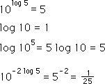
Before moving into the development of our equation, let us review some basic rules. Because we have been speaking about logarithms and exponentiation let us first just review a few of the rules that govern their behavior.
Let us start with exponentiation.
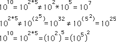
Let us briefly note that the commutative property does not apply to the property of exponentiation. This is shown clearly in the first three equations. Thus the placing of the parentheses in exponentiation is crucial.
Below are some of the definitional rules of logarithms.
Note that a negative logarithm represents an inversion.
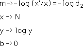
Now that we have reviewed a few of these basic relations we can move on to the classic representation of the line equation. Shown below.
While x & y are variables, m and b are constants. The constant m is called the slope of the line. The slope of our logarithmic line is the negative of the Log of the Divine Ratio, m -> -log (d2). This was illustrated clearly in the just mentioned computer experiment. The Divine Ratio we shall call d2, for reasons that will become apparent later on.
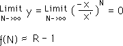
This means that for each iteration N, that our value for ƒ(N) becomes closer to Limit, which is the Square Root minus one. It becomes closer by a distinct increment which is the log of the Divine Ratio, -log (d2), For each iteration our Root Being takes a logarithmic step closer to the Limit. Thus N, the number of iterations, is the variable that drives the equation and so would be the X in the above equation, x -> N.
Turning the y-axis logarithmic was what straightened out our line, thus the y value is represented as a logarithm. Thus we can represent the y in the above equation as y -> log y. The value of the y-axis, which corresponds with each iteration, represents logarithmically how close our iterated function is to the Limit. Thus as our graph ‘moves’ to the right, the negative exponent that represents how close we are to the limit gets larger and larger. Remember that as N approaches infinity that log y approaches negative infinity. This means that the limit of y is simply zero, because this is the Difference between the F Series and the Limit. In crude terms: When N is infinity the F Series equals the Limit. Thus their difference, i.e. y, equals zero. But for our graph, we are talking about the logarithm of this difference, it becomes a very big negative number, eventually approaching negative infinity.
The constant b is called the y intercept, because it represents the value of y when x or N, the number of iterations, equals zero. This point doesn’t really exist, although it could be projected. However this point doesn’t really matter. Because we are getting closer and closer to the Limit with each iteration, it doesn’t really matter where we start. Because of the nature of our iterative expressions the beginning doesn’t matter. We become logarithmically closer with each iteration in a linear fashion. Thus although the starting point could definitely slow us down in our Quest, it could certainly not deter us. No matter where we start, we will take these consistent baby steps towards our goal. Thus in the derivation that follows we will let b = 0, because the value has no real meaning anyway and this makes our equation of a line the simplest.
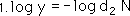
These substitutions are shown all together below.
Now let us drop these expressions into the equation for a line and see what we’ve got.
This equation states that the log of the Difference between iterated function and its limit is equal to a linear function of the number of Iterations, N, where the slope is -log d2.
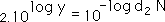
Of course like any good mathematician, we need to raise all those logarithms to the 10th power to clean them out.
First 10 raised to the log y power equals y. Shown below. 2nd: The negative in the exponent on the right means to invert. Therefore we place the expression in the denominator of a fraction, simultaneously eliminating the negative sign in the exponent. Further we invert the exponential product for clarification.
This expression converts easily to the following simple expressions.
Now that we are out of logarithms, we can remove the absolute value signs that should have surrounded d2. Below is the real expression for d2., complete with negative sign.
This negative sign is very helpful for expressing our true graph because now the function bounces back and forth between a little above zero to a little below zero. Remember that y equals the difference between the iterated F Series and the Root minus one, of any square root. As N, the number of iterations approaches ∞, y, the difference, approaches zero. The equation below approximates our Difference Series, i.e. the difference between the F series and the Root minus one. Remember that the Divine Ratio between the parentheses is only an approximation of the slope as N approaches infinity. But we saw that it was a pretty good approximation.
Thus far our equation from step 6 only describes the behavior of our function in the realm of real numbers. Now let us move into the imaginary world.
In the above equation, N is restricted to being a positive integer because N represents distinct iterations. Thus y, which represents the Difference Series, is only a set of points, not a continuous curve.
Indeed the Fraction Series, which the Difference Series is based upon, is itself only a set of points that approaches the Root minus one as a Limit. Indeed some of the points are greater than the Limit and some are less than the Limit. When we graph the Difference Series, which is the difference between the F Series and its Limit, i.e. the Root minus one, the individual points converge rapidly, bouncing from over to under zero. If however we graph this difference from a logarithmic perspective, we see a line of points. The visuals for this phenomenon were seen at the beginning of the last section.
What happens to our Difference Series between these iterative points? We are going to postulate the existence of a continuous function that moves in and out of the real world from the imaginary world. The points that appear in the real world exist only because the imaginary component equals zero.
This is a common mathematical phenomenon. Indeed Stephen Hawkings postulates in his book, a Brief History of Time, that the real universe is only expanding into the imaginary universe, but that the combination of the two is a constant. When the real universe starts shrinking then the imaginary universe will begin growing. The Big Bang occurred when the real component of the Universe was nearly zero. Anyway this section is looking for the equation that will represent our distinct, discrete F Series of real points from the continuous perspective of the Complex world.
This is also a common phenomenon behind consciousness also. We are truly aware of the Present in discontinuous segments, fragmentary at best. These experiences of Being are separated from each other by the imaginary world of thoughts. These thoughts create an incredible imaginary world of desires, fears, pain and pleasure, questing and dissipation. Every once in a while the world of thoughts is forced back into the Now for brief moments to deal with Reality. Over all, however, the thread of our connection with the Now of the real world is connected by imaginary thought projection. Thought projection is not ‘evil’, or even something that needs to be resisted. It just needs to be recognized as the false. It just needs to be differentiated from the ‘real’ of Being. Cultivate the real and the false will naturally melt away, exposed to the light of consciousness.
Our Difference Series for Square Roots could be seen as representing the points of real between the imaginary. Thus the Difference Series could easily be represented by a simple complex spiral, whose ultimate limit is zero. Thus it spirals from a little above zero, to a little below zero, to a little closer above zero, to a little closer below zero. As mentioned the continuity is furnished by imaginary components. When the imaginary components equal zero then this proposed continuous function approximates our Difference Series values.
In the previous discussion N, represented the number of iterations and thus was a distinct whole number. Let us allow N to move continuously instead of in distinct steps. We will assign it a new variable, theta q. Further we will let it move in and out of the real realm by assigning the following value to N.
With this substitution N is only completely real when q is an integer. When q is not an integer, the imaginary component, i sin πq ≠ 0, is not equal to zero, but when q is an integer then the imaginary component, i sin πq = 0, equals zero and disappears. Further because N is always positive we must square our trigonometric components, i.e. the cosine and sine functions, to balance things out. When q is an even integer then cos πq always equals one and sin πq always equals zero, neutralizing the imaginary component. However when q is an odd integer then cos πq equals -1 while sin equals zero. We don’t want our function to be negative so we square our cos and sin function.
We have assigned a continuous function, ƒ(q), to the number of iterations, N. We show this substitution into equation 6 in equation 8 below, where y is a function of q rather than a function of N.
In step 9, we merely show the expanded version of the same ƒ(q), defined in step 7.
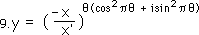
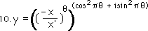
In step 10 we apply the law of exponents again to get our final representation of the complex spiral that we were aiming for.
What does our equation of the Complex spiral do? It spirals ever closer to zero in geometric increments. What does it look like?
From the real perspective, our equation for y above would only be a few points that quickly reach zero. (We saw this graph at the beginning of Section 3, entitled The Slope.) From a complex perspective the graph looks like a spiral on a funnel, which quickly reaches zero. Remember this zero is the Difference between the F Series and its Limit, the Root minus One. The bottom and top most points of our spiral both form sharp curves like a roller coaster, which start sharply down or up and then quickly level out. When our top and bottom curves level out they intersect at zero.
From a logarithmic perspective of the real world, again we have two series of points, both suggesting lines, which intersect at zero. From a logarithmic perspective of the complex world our graph is of a spiral that gets progressively closer to zero. This perspective is shown below.
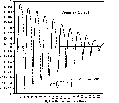
Note that while the spiral seems to moving quickly towards zero that it actually never reaches there. We have truncated the logarithmic region between 1.0 * E-16 and zero for purposes of display.
In the next graph we show the Implied Lines of the Complex Spiral. The points where the Lines intersect the Spiral are the F Series iterations; the rest of the graph is only the imaginary projected upon the real for understanding.
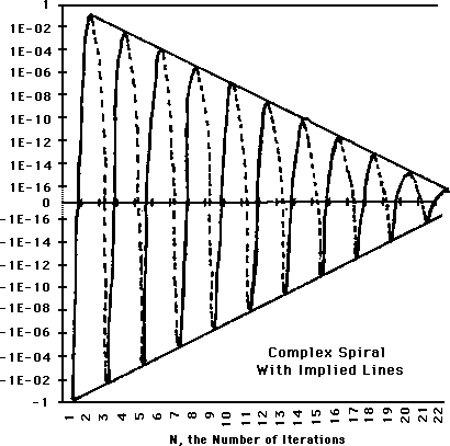
Our logarithmic graph is shown from a complex perspective. The points are real. The curves from the points move into the imaginary realm. The lines, except for the points, while existing in the real plane, are pure projection. Remember that the complex perspective includes the imaginary world, while the real world does not.
The two implied curves of an ordinary perspective intersect rapidly at zero. From a logarithmic perspective these curves turn into two implied lines, which never intersect, no matter how close they seem to get. It is a spiral that moves continuously inwards. The top and bottom points of this spiral form two lines that point towards zero but never actually reach there. Their imaginary point of intersection is emptiness, nothing, zero. Note that the implied lines of the real world don’t even exist in the complex world. All the motion from one point to the other happens in a spiral fashion from the imaginary world rather than from a linear fashion in the real world.
Taking a step back. Note that our simple number has now become a bounded spiral, moving through the complex plane, in and out of the real plane. Each time it reaches the real plane, the F Series for square roots, which is itself a function of a D series, can characterize it. Our number doesn’t really have a Limit in the ordinary plane. The spiral moves continually inwards, never reaching the center.
Now that we have explored the physical attributes of our Complex Spiral, let us explore the metaphorical and metaphysical implications of our equation.
What appears as two sets of discontinuous points from the real perspective, actually could be described as a single spiral from the complex perspective, which combines the real and imaginary worlds together in a single plane. Thus it is many times with our mind. Our thoughts break the world into many seemingly discontinuous parts. Further because our rational mind can only perceive the real world and not the imaginary, it firmly believes that the world is truly broken into an infinity of different and conflicting pieces, which align themselves in a chaotic and seemingly random pattern.
However in the transcendence of thought in the perception of the world, the imaginary realm connects the physical world together in the complex plane, which combines the real and the imaginary. Suddenly all that made no sense to the mind, because it is broken into real parts becomes connected by our imaginary spiral in the complex plane. Further our logical mind cannot even begin to perceive what this imaginary world consists of. Our minds cannot hope to perceive what it means to be the square root of negative one. All we know is that the imaginary plane bonds the real plane into the complex world in a continuous fashion. Thus the first metaphorical lesson to be learned is that thoughts limit direct perception.
A second lesson has to do with the depth of perception influencing the appearance of reality. Sometimes reality will even be perceived in diametrically opposite ways. Those seeing our graph from an ‘ordinary’ perspective see a bunch of points that converge quickly. Those who are able to see into the complex plane logarithmically see a Complex Spiral moving ever inwards. The ‘ordinary’ perspective turns the world into positive and negative polarities, while the ‘special’ perspective sees an unbroken continuity of perspectives. In this ‘ordinary’ worldview distinct goals are stressed over the continuity of process.
Another flaw of perception that is revealed in our equation and graph has to do with the concentration of perspective. Many have only cultivated a linear perspective. Under this perspective, our graph reaches its goal quickly, while under the more concentrated perspective, the goal is never reached. From a linear perspective the iterations quickly reach the goal, while from the more concentrated logarithmic perspective, the goal is always infinitely far away. From the linear perspective, enlightenment is the end goal to be reached, while from the logarithmic perspective, it is merely a step along the path. From the linear perspective the students movements fairly quickly intersects the line of the Master, while from the more subtle logarithmic perspective, the Master’s movements are incomprehensibly subtler. From the perspective of the novice student, the Master is enlightened, while from the Master’s perspective he has a long way to go.
Initially our student/observer’s perceptions are very blunt because they have not been cultivated. They might even think that their movements converge with the Master. They feel a sense of false confidence. When our student increases the depth of his perception, two things happen in this metaphor. Huge gaps appear between the end points of his mini-goals and the end suddenly seems increasingly further away. The chasm of uncertainty opens up, which eventually leads to a deeper understanding. Thus a blunt self-confidence has been replaced by a more subtle humility. This is called going backwards to go forwards. Pay attention to this mechanism and cultivate its perception .
When the student cultivates his perceptions and reaches the above ‘enlightenment’, he sees something radically different to what he saw before. With his goal-oriented mind, he saw only two quickly converging curves. Now with increased perceptions he sees that his curves are only a series of distinct points. Further a chasm has opened up between the end points of his curves, which have turned straight. Thus the ‘truth’ of two converging curves has been replaced by the ‘truth’ of two straight lines, which are not continuous at all but consist merely of points. Further these point lines never converge. Thus the phenomenon is the same, but the level of perception yields up two contradictory notions of truth. The lesson here is that an increase in perceptions can lead to transcendence of the ordinary realm. The difference is not just a matter of degree, but is an emergent property of perception.
With this enlightenment based upon increased perception, the student comes to realize that his notion of truth has transcended that which went before, while still including it. Hopefully the student gains humility from this transition, not pride. If he holds onto his emergence as a new truth that he has gained, he will probably feel pride. However if he realizes that this emergence will only be followed by more emergent truths as his perceptions increase then he feels a great humility before the awesomeness of it all. Now our student might be able to perceive that while they are on the same Path as the Master that his refinement far surpasses what they have achieved. At this point they have made a huge step forward and are able to comprehend refinement.
Our Student has increased his perception from a linear to the more concentrated logarithmic perspective, but has still not increased the depth of his perception to include the imaginary world. While our student has increased perception, he has not yet let go of thought as his mode of apprehension. Thought based in polarity does not include the continuity of the complex realm. As the Student’s perception is focused inwards, thoughts are dissolved and experiential reality emerges. Because experiential reality is so spontaneous, the inner subtle circles might manifest unexpectedly and possibly even erratically in the exterior world. Thus we arrive at the converse. Those, who haven’t developed their perception thoroughly and can only see through their eyes rather than their intuitions, might see internal continuity as external discontinuity. Of course the Master disguises the internal spontaneity as external continuous movement further tricking those that can’t see. Advanced students might be seen as raw beginners, while intermediate students might be perceived as next in line to the master.
Thus the perception must increase to apprehend the imaginary world of internal movement in order to integrate mind and body on the highest levels. Remember however that the perception of this imaginary realm must be sensed intuitively. It cannot be directly perceived by thoughts and analysis. This is simply too slow and discontinuous. Thus while thoughts might act as a bridge to the experiential level of internal movement, they must be abandoned when you get there.
Further the mind must be continually be purged of thoughts in order to stay in the experiential realm. Thoughts, because they break things into pieces and separate observer and observed – experiencer and experience, are necessarily discontinuous. Further because of the back and forth between mind and experience, it is far too slow, blocking direct perception of reality. The mind while a great signpost is incredibly limited in the perception of experiential reality and must be abandoned.
Now that thought has been purged and our student is able to perceive reality from the complex plane, he now sees the two lines of points as an infinite spiral moving continuously in the complex realm. Therefore another level of truth has emerged which is seemingly contradictory to the level of truth that went before, but which transcends and includes it. Increasing the level of non-verbal perception is essential for this next step.
Before getting carried away let us remember that this whole section on the complex spiral is metaphorical in nature.
The F Series data is real. The differences between the F Series and its Limit, the iterated Difference Series, are also real. Each iteration drives the function closer and closer to the Root in a logarithmic fashion. While these points are real and exact, the visual line that connects these iterative points is imaginary and approximate. While our line has a 99.995% correlation with the data, it is not exact. Thus our line is not the ‘real’ line. It only represents a best-fit line, as in statistics. That is why we compared it with the best-fit line from statistics in our earlier analysis of the chart. Therefore the only thrust of this section was to write an approximate equation that would describe our Difference Series for square roots in complex terms.
This leads us into the topic of differences between ‘ordinary’ equations and iterative equations. With ordinary equations they are either right or wrong. Using ordinary equations to describe iterative equations is a hopeless task. They can be more or less right but can never be completely right, because even at the most fundamental levels the slope of the iterative line is only approximate. That these iterative equations generate lines at all is miraculous, that we could expect to have an ordinary equation describe this linear relation perfectly is a little much to ask.
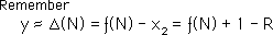
To be a little more specific, let us look at some algebra. Remember what y represents. It is supposed to emulate the Difference series, ∆(N), just as a physics equation attempts to emulate the ‘real’ world. Note that the Difference Series is the difference of the F Series and the Limit, which contains the Root.
To simplify let us look at our equation for y without the imaginary components, equation 6. If y ‘equals’ this exponential ratio then it only approaches the Difference Series as a limit because the slope is only based upon a limit also.
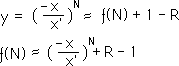
Using some elementary algebra we rewrite the first equation in terms of ƒ(N).
We remember that the limit of y as N approaches infinity is zero. Thus the relation between the Root and the F Series is independent of the components of y.
With this representation it is obvious that while ‘y’ contains both ƒ(N) and R, the Root Number, it in no way assists us in the computation of ƒ(N) or the Root Number, R. It just approaches zero as N approaches infinity. But it gives us no clue as nature of its components. The ordinary equation, i.e. with y, must base its result upon the answer, i.e. the Root, while the F series is independent of answer.
Thus our complex spiral will not help compute the Root, while the F Series heads inexorably towards the Root no matter what nonsense is fed into it. Therefore the F Series never gets lost while the ordinary equation must align itself with the master symbolized by the Root. The F Series is guided by an internal pattern and doesn’t need the Root to find its way. It can never get lost. Conversely the ordinary equation for y needs the Master Root for guidance.
In this case an ordinary equation is a content-based equation, while our iterative feedback equations are context based. An ‘ordinary’ equation yields the same instantaneous answer, after the numbers are plugged in for the variables while with the iterative equations one must ask how many times it has been iterated to get the right result. One can ask the question where an iterative equation is going while ordinary equations are already there. Therefore iterative equations grow, while ordinary equations are static. Thus ordinary equations are ideal for describing ‘dead’ phenomenon, i.e. those based purely in the physical realm. Contrarily, they are hopelessly inadequate for describing ‘live’ phenomenon. On the other hand the context-based iterative equations are unnecessarily animistic when describing inanimate objects, while their growth patterns are ideal for mimicking and describing context-based situations, where the result is determined by the situation rather than some absolute answer.
Thus bear in mind that in this section we are attempting to use an ‘ordinary’ equation to describe an iterative phenomenon. Our search is ultimately futile except as a metaphor. However the result that we achieved was so beautiful that it is tempting to assign reality to it.
This is the last level of metaphor. Basically the complex spiral metaphor, which seems so beautiful, which reflects the reality of the F Series so accurately, is only an imperfect reflection. It is the same with words or thoughts. No matter how closely words or thoughts reflect reality, they are only a metaphor, which is not quite reality. Our complex spiral with all its metaphorical significance is only a pale and dependent reflection of the reality of the F Series. The F Series really approaches its Limit, while the complex spiral only emulates the approach. The beauty and regularity of the complex spiral is attractive, safe and secure, and probably most importantly, understandable. It is a content-based equation, which is static. Our real context based equation, the iterative F Series, is based upon ambiguous shadings and half steps. It doesn’t need to focus upon its goal. Through a constant balancing it proceeds inexorably towards its Limit, independent of input. Thus the complex reality of this iterative process is made more understandable by the complex spiral. But the understanding while assisting our conception is not really true. In this metaphor, the F Series represents Reality, while the Complex Spiral is but a beautiful reflection.
Let us review a few of our discoveries concerning the nature of the F&D Series’.
In looking at the family of numbers in the infinite continued fractions, there are some interesting conclusions that can be reached. First there is an infinity of points between any 2 numbers. As mentioned earlier, the odd functions are below while the even functions are above the square root. Hence the square root of any positive rational number, which includes positive rational numbers, exists only between even and odd. Because nothing is there, there is always an infinity of points between a little more and a little less. Each number is only an approximation. One can become as precise as necessary but one can never reach between even and odd. Our ideal number behaves as a practical magnitude. We are back where we started.
We discovered in this Notebook that: Given any rational number, X, a series can easily be written, such that the ratio of consecutive terms approaches the square root of that rational number. Written another way, any square root can be written as the limit of the ratio of consecutive members of an integer series. The irrational square root can be written as the limit of a ratio. This is just the beginning.
This integer series, which we call the Denominator Series or D Series, is generated by self-referencing the last two members of the series in a specific way. However the pattern is so dominant that the first two members of the series are inconsequential to the inevitable result. Hence the pattern becomes more important than the numbers used to begin the series. Number fades in significance to Pattern as determining the identity of the approximate number. Because of the supremacy of the pattern of the D Series for determining square roots, we decided to look a little more closely at the pattern. In looking at these patterns, we found an incredible underlying structure, where coefficients became elements of the D series.
Because of all these marvelous connections and discoveries we are craving an exploration of the Higher Roots thru’ the glasses of the Infinite Continued Fraction Series and its derivative, the Denominator Series, i.e. the F&D Series. We don’t know if there is any connection and if there is any connection what it is. Onward to the next Notebook, Higher Roots, to find out.